• About Jam on Toads
• Luma & Chroma Waveform Emulation

Luma & Chroma Waveform Measurements and Emulation

Introduction

I spent a month or two back around the start of 2015 measuring the composite video output of my c64 using a 100MHz USB oscilloscope (a SmartScope from LabNation), then trying to reproduce the output waveform using a simple predictive model.

Before I started, I had this crazy idea that I could use the fragments of chroma signals from each pixel to manufacture new colours, on the assumption that each pixel would be a well defined slice of a sinewave. Ahahahaha. Nothing so simple. Chroma takes several pixels to start up and shut down again, and the luma signal rings visibly for four or five pixels.

I do now however have a pretty accurate model of the luma behaviour, and my chroma model is not far off.

Test assumptions

I also assumed that the signal produced is purely dependent on the ‘ideal’ pixel colours, and the position relative to the colour burst; eg, a sprite pixel is the same size and shape as a character foreground pixel, and there are no transition effects from any VIC state changes beyond the desired output colour. This is patently untrue in the case of (eg) the ‘grey dots’ you get from changing $d020 from black to black, but that’s an issue for another day.

These assumptions did allow me to create test patterns with relatively mild colour restrictions by overlaying a number of hires sprites over a hires bitmap.

Measurements

My ‘scope contains enough RAM for a good chunk of a frame, but the firmware at the time of my testing only allowed me to capture a raster line or two, so each test was performed by displaying a single line of pixels on an otherwise black screen.

Every test had a black border, with a couple of white pixels at the start of the line for synchronisation. This way I could trigger on the first rise past 0.8v, but use the scope buffer to record from a few microseconds earlier to ensure I also record the colour burst as a reference for the chroma signal.

Each test I grab a few hundred recordings, then for each recording filter out frequencies above about 8MHz, set the start time to the point the signal starts responding to the the first white pixel, resample to 18 samples per pixel, then take the mean of the aligned recordings and cache the averaged sample for analysis.

The first suite of tests was designed to purely investigate luma changes without any interference from the chroma circuit, and I’ve now got a model that can predict the luma behaviour pretty closely.

For some reason I could not measure the chroma output from my c64 directly, so for chroma modelling I just measure the composite signal, subtract the predicted luma, and then attempted to fit a model to the derived chroma.

The entire suite of tests was performed without power-cycling my c64, so that I could assume the colour burst phase relative to line start was consistent for every test – sadly not something that can be guaranteed across power cycles.

All colour measurements were performed on both odd and even lines, and in each case the phase was measured relative to the colour burst at start of the line.

I made heavy use of De Bruijn Sequences to allow me to test every possible substring of small subsets of colours, while still fitting within my 160 pixel test window, and also some random strings.

Model output

You can see here the first 16 pixels of a 7th order De Bruijn sequence of white and black pixels, namely a run of 1111 1110 1111 1001. The measured signal is shown in green, and my model’s prediction is shown in red. The grey rectangle wave shows the ideal luminances.

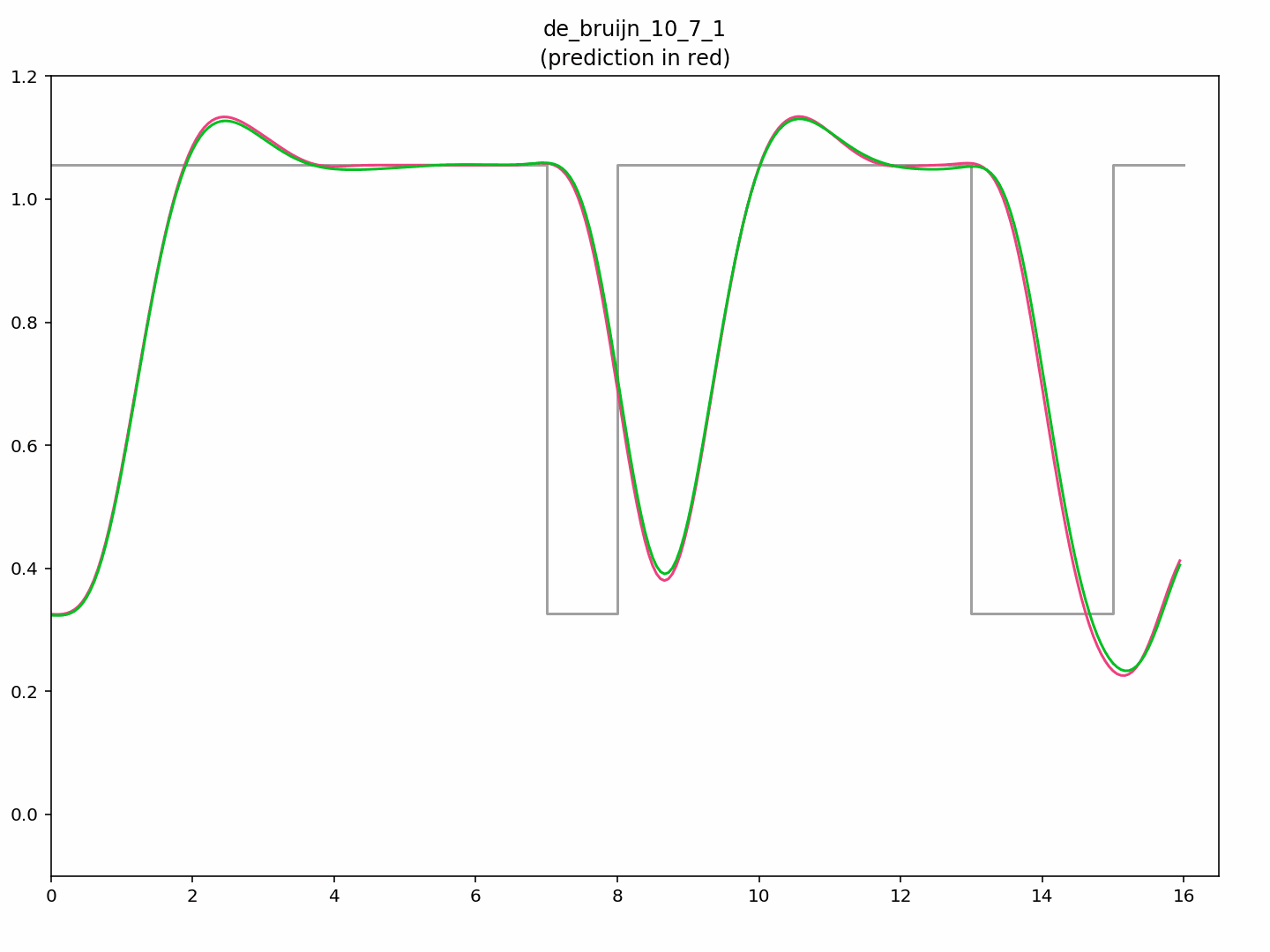
Note that the nominal black voltage is 0.32v, nominal white is 1.05v. The c64 takes almost two pixels to reach 1.05v, then overshoots to about 1.14v before settling. It’s attempt to display a single black pixel spends 1.5 pixels worth of time dropping almost to black, before spending the same again to return to white, and overshoots once more.

Here’s a more complex signal, featuring runs of four pixels from a palette of black, grey 1, and white:

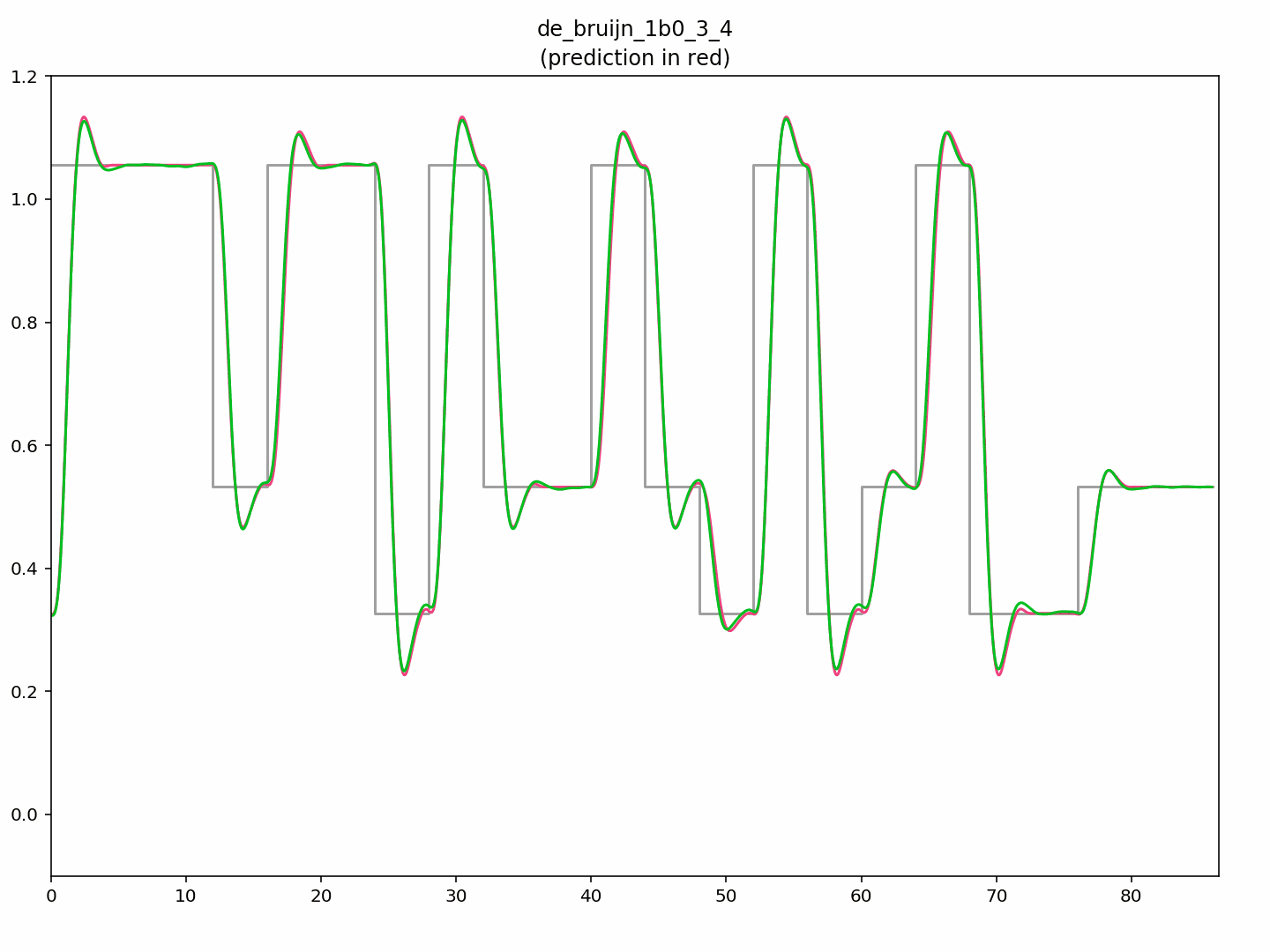
Again, the model follows the measurements reasonably closely.

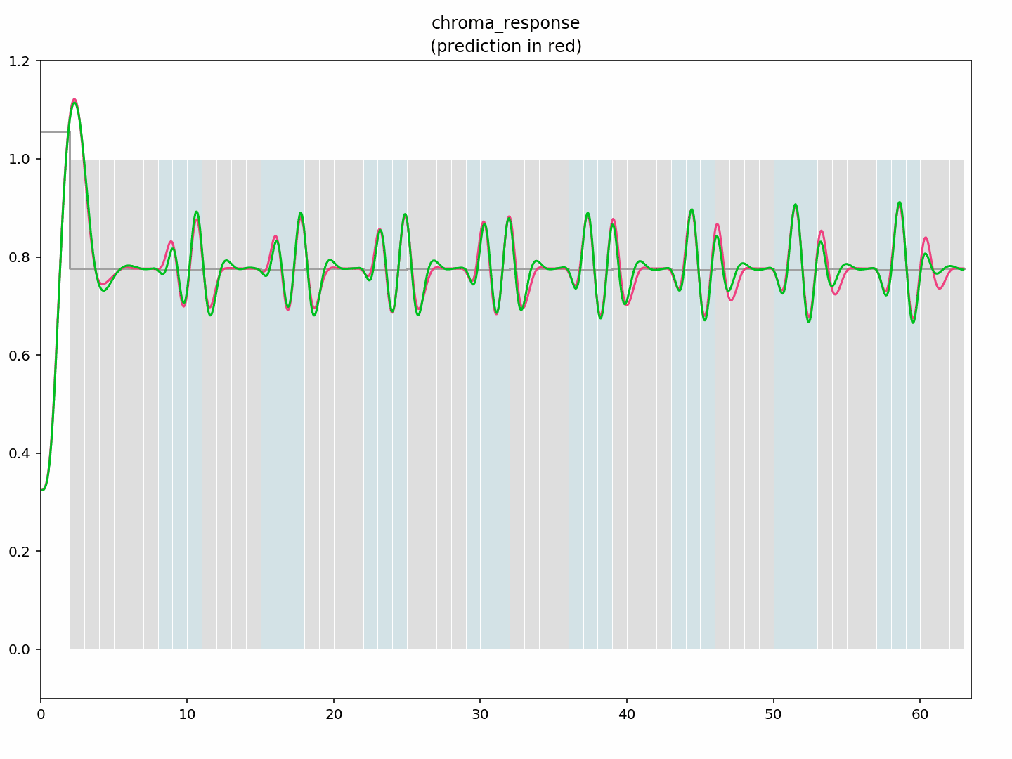
Getting a good fit for chroma has proved to be more difficult. Best I’ve managed is a quadratic form whose inputs are the magnitudes of the sine and cosine components of the idealised versions of each of the last four pixels. As you can see from the measurement and prediction below, chroma responds more quickly than luma, but there’s still a startup delay when going from a grey to a colour, and the transitions between colours are similarly sluggish.

Initial test – a repeating sequence alternating six light grey pixels with three cyan pixels (fff fff 333), allowing luma to be ignored completely, while capturing sixteen different startup phases in a 144 pixel window. I’ve shown the first eight groups.

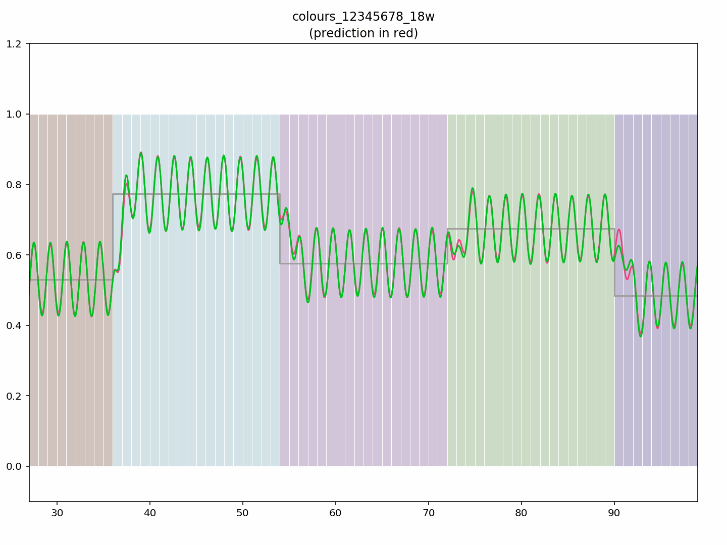
A nice colour bar, with a couple of red pixels preceding a ramp up from black through browns and yellow to white
(1, 1, 0, 0, 2, 2, 0, 0, 0, 4, 0, 9, 2, 8, 12, 10, 15, 7, 1, 7, 15, 10, 12, 8). Again, measurement in green, prediction in red, ideal luminance in grey.

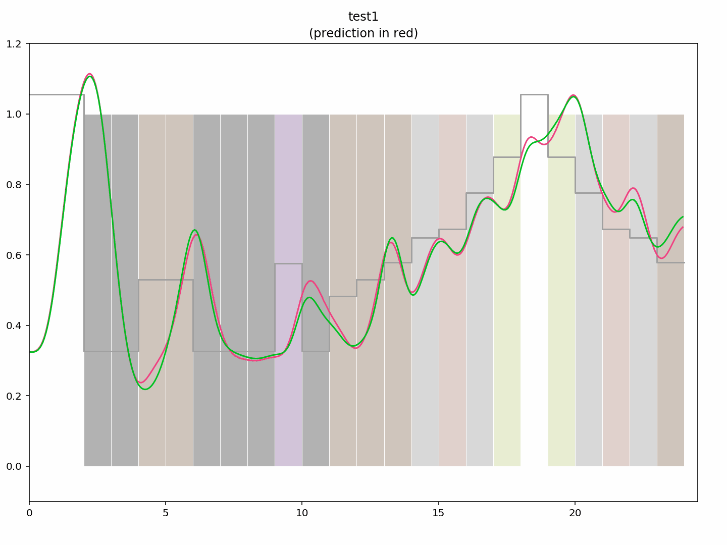
You can see the transitions still need some work, but it’s not too far off.

The modelled steady state chroma response at least is a very good fit to the measured data, and is easily sufficient to produce a new palette. Here are some groups of 18 pixels each of red, cyan, purple, green & blue:

..and here’s a palette generated from the steady state of the model output (so, basically the measured colours):

jampal=[000000, ffffff, 7d202c, 4fb3a5, 84258c, 339840, 2a1b9d, bfd04a, 7f410d, 4c2e00, b44f5c, 3c3c3c, 646464, 7ce587, 6351db, 939393]

Results

I’ve used the models referred to above along with some composite video to YUV to RGB converters (yes, including UV averaging) to make a proof of concept image converter. As is, it is far too slow to incorporate into an emulator, but I’ve already done some experimentation with table driven approximations to the model. More on that later.

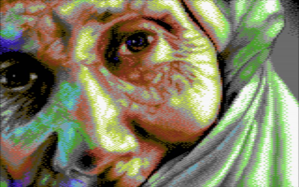
I’ve included four test images below; mouse over each one to see a naive conversion that just uses a pepto palette then applies a gaussian blur.

Looking at these test images, it’s interesting to guess which artists were working on a real c64, and which ones were working on a cross platform editor;

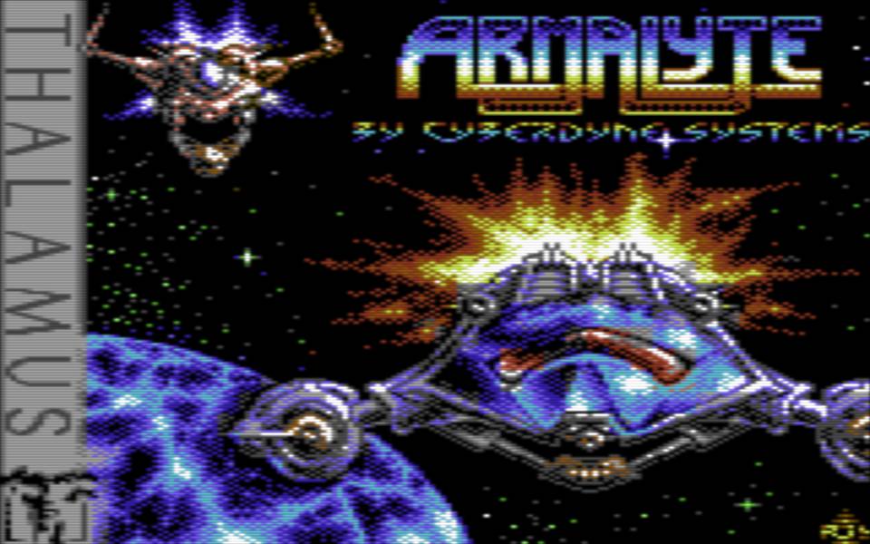
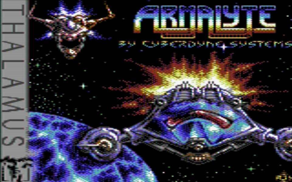
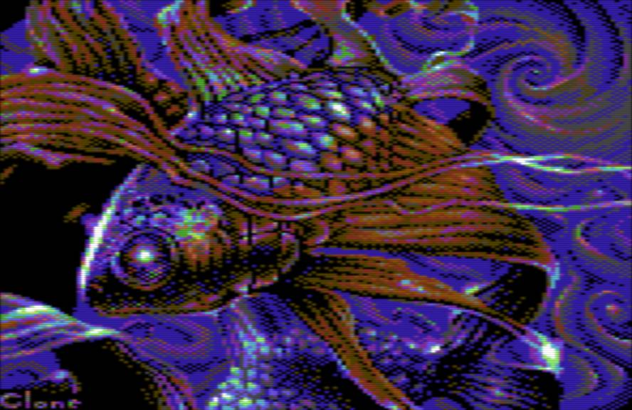
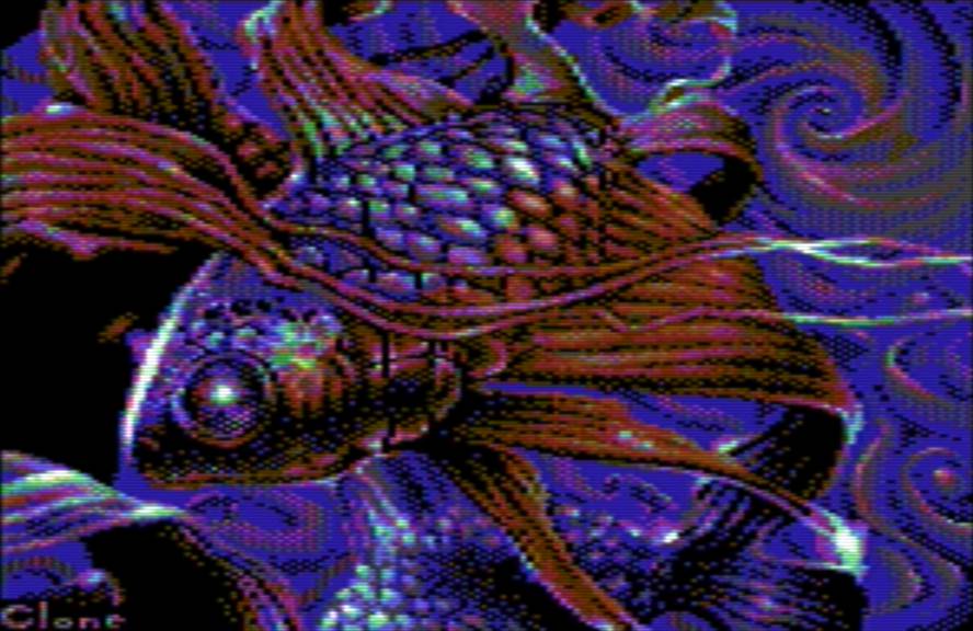
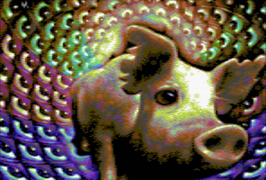
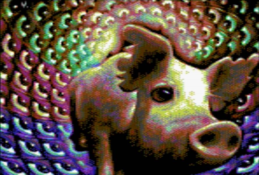
Armalyte and Fish definitely benefit from the improved luma simulation; check out the antialiasing around the engine nacelles in the Armalyte pic and in the fine strands in Fish. Wool doesn’t gain so much; it’s a slightly different palette, but it looks no better than the naive conversion. Pig on the Wing I wasn’t sure about; try and guess before you go read the production notes at CSDb.

Armalyte loading screen

Fish by Clone

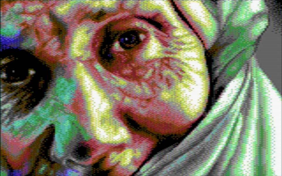
Pig on the Wing by Valsary

Wool by Cosine

Future plans

So, I’ve currently got a python library that churns through about 4MB of oscilloscope traces, and crunches that down to about a dozen kB of cached model parameters, which it can then use for output prediction. I’ve just ported the library from python 2 to python 3 few days ago (late October 2017). I’m not sure how much interest there is in the raw measurements, or whether to just put together a smaller library with the model parameters baked in.

There’s also a somewhat less accurate table driven approximation I’ve thrown together for an image editor I’m working on. More on that when I release the bastard.

If any of these interest you, give me a shout on CSDb or Facebook, and I’ll see what I can do. Meanwhile, the palette I gave above is excellent, you should all use it.